On the weekend I was playing snakes and ladders with my sons. Since it’s a game without any element of skill, and relies completely on the roll of the dice, I haven’t played the game for about as long as I can remember. The first game we played was over pretty quickly, but the second lasted for what seemed like an eternity, and well past the endurance of the boys’ attention span. As one of us got near the end, we landed on the final snake.
Frustration waxed; interest waned.
Eventually I employed the parental right of rigging the dice throw so that the game mercifully ended, and we could move on to something a bit more interesting (like Castle Logix - really clever design).
Anyway, I began to wonder what the probability was of playing a game that went on that long. Since there is no human decision (skill) involved, it should be reasonably straightforward to run some simulations and get some answers.
I’ve also been wanting to get a bit of practice with purrr, Hadley’s functional programming package. So, what follows is at times probably more complex than it could be, but represents my learning process, and is one approach to managing data in a bunch of nicely organised lists.
The first step was to represent the game board we were using. You’ll notice it’s heavier on snakes than ladders!
Firstly to define the snake and ladder positions and effects:
#Define the starting location of the snakes
snakes <- data_frame(square = c(19, 24, 28, 34, 40, 49, 55, 59),
                     effect = c(-15, -15, -15, -14, -24, -12, -13, -14))
#And the ladders
ladders <- data_frame(square = c(2, 6, 22, 30, 38, 43),
                      effect = c(13, 15, 14, 11, 20, 14))

snakes_ladders <- bind_rows(snake = snakes, ladder = ladders, .id = "type")
Next to define the board layout - game play progresses in serpentine fashion (appropriately). This includes the dimensions, the order of progression through the board, and adding the snakes and ladders.
board_layout <- data_frame(square = 1:60, y = rep(1:10, each = 6)) %>%
  group_by(y) %>%
  mutate(x = ifelse(y %% 2 == 1,
                    1:6, 6:1))

#Add snakes and ladders to the board
game_board <- board_layout %>%
  left_join(snakes_ladders) %>%
  mutate(effect = ifelse(is.na(effect), 0, effect))

#Get the finish position of snakes and ladders, and tidy
effects_df <- snakes_ladders %>%
  mutate(id = 1:nrow(.),
         result_square = square + effect) %>%
  gather(start_result, square, square, result_square) %>%
  select(square, id, type) %>%
  left_join(game_board %>% select(-type))
To check it’s all making sense, I’ll compare the virtual board with the physical one. Notice I changed the numbering since the board makers decided to use zero-based numbering…

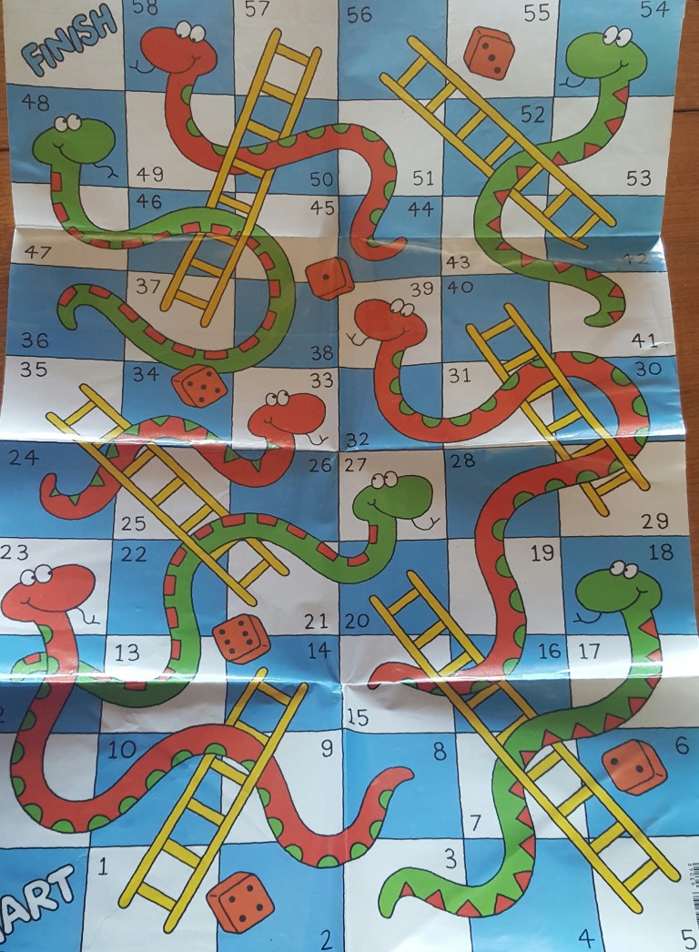
The actual ‘board’
Maybe not a marketing success, but functionally the same.
Next I needed to make some functions to simulate the players and the turns each players takes.
There would be lots of ways of doing this, but I decided to represent each player as a list object made up of vectors representing the position in which the player finished each turn, and another vector representing the full path they took (including traversing snakes and ladders). Each game would then be structured as a list of the player lists.
Since I can’t predict the number of turns, I can’t pre-allocate the vector length, and so we enter the second circle of the R Inferno by growing these objects, but since they’re pretty small I hope you’ll forgive me.
#A function to make a list of players
make_players <- function(n) {
  players <- map(1:n, function(x) list(sq = 1, path = 1)) %>%
    setNames(paste0("player", 1:n))
}

#A function to represent a turn
turn <- function(player, effects) {
  sq_i <- length(player[["sq"]])
  path_i <- length(player[["path"]])
  roll <- sample(1:6, 1)
  sq_temp <- player[["sq"]][sq_i] + roll
  effect <- effects[sq_temp]
  if(sq_temp < 60) sq_new <- sq_temp + effect
  else sq_new <- 60
  player[["sq"]][sq_i + 1] <- sq_new
  player[["path"]][path_i + 1] <- ifelse(sq_temp > 60, 60, sq_temp)
  if(effect != 0 & !is.na(effect)) player[["path"]][path_i + 2] <- sq_new
  return(player)
}
I’ll check the functions by making a very simple simulation:
players <- make_players(2)
players
## $player1
## $player1$sq
## [1] 1
##
## $player1$path
## [1] 1
##
##
## $player2
## $player2$sq
## [1] 1
##
## $player2$path
## [1] 1#Each player starts at square 1
turn(players[[1]], game_board$effect)## $sq
## [1] 1 5
##
## $path
## [1] 1 5#The function is returning player1's list after their first turnSince the path vectors of the different players aren’t necessarily the same lengths (since it will be longer for each snake/ladder), I needed to be able to pad the vectors with NA. This is something that doesn’t seem to have a straightforward, canon approach, so I made a little function to deal with it.
pad_na <- function(vec, length) {
  if(length(vec) < length) vec[(length(vec) + 1):length] <- NA
  return(vec)
}

pad_list_na <- function(list) {
  max_length <- max(unlist(map(list, length)))
  list_out <- map(list, pad_na, length = max_length)
}
And now the function to actually simulate a game. This needed to take the number of players and board layout, give each player a turn until one of them reached the finish, and then return each player’s locations throughout the game, as well as their path.
This brings me to list columns - the element of dplyr’s do and purrr output that I’ve found most challenging in the couple of months I’ve played around with them. List columns are incredibly powerful, meaning you can store dataframes, models, figures, anything. So instead of having a pile of lists cluttering up the workspace, these objects stay neatly arranged with the structure from which they were created.
That being said, trying to deal with those columns has made me feel like:
And I’m clearly not the only one, given some of the conversations that have happened in #rstats
@noamross @polesasunder I am actually planning to teach dplyr::do() tomorrow and I'm, like, what do people do with these list-columns?!? 😯
— Jenny Bryan (@JennyBryan) October 13, 2015
So far I have relied more or less completely on broom (which is brilliant in lots of situations) for dealing with list output from dplyr::do(), but there’s often a lack of flexibility. I think this is where purrr is the knight in shining armour.
In this game simulation function each player’s list takes a turn until one of them reaches the finish. The lists are then transposed to allow each players position and path to be made into a dataframe, and these dataframes are then returned in a list. Using mutate lets me add the list for each simulation into a new column.
sim_game <- function(n, board) {
  players <- make_players(n)
  while(max(unlist(flatten(players))) < max(board$square)) {
    for(i in 1:n) {
      players[[i]] <- turn(players[[i]], board$effect)
    }
  }
  players_tr <- players %>%
    transpose()
  sq_df <- players_tr[["sq"]] %>%
    as_data_frame %>%
    gather(player, square) %>%
    mutate(player = sub("player", "", player))
  path_df <- players_tr[["path"]] %>%
    pad_list_na %>%
    as_data_frame %>%
    gather(player, square) %>%
    mutate(player = as.numeric(sub("player", "", player)))
  # return(sq_df)
  return(list(sq = sq_df, path = path_df))
}
The structure of the complete simulation can then be setup in dataframe, where each row represents the parameters to be used for each game. I’ll run 2500 simulations for 2, 3, and 4 players. I get the output column (recall it’s a list of two dataframes), and then separate these out into their own columns. That’s inefficient, but convenient in this case. I’m also calculating the number of turns for each game and making a new column for that as well.
game_df <- data_frame(game = rep(1:2500, 3), players = rep(2:4, each = 2500)) %>%
  rowwise() %>%
  mutate(output = map(players, sim_game, board = game_board),
         sq = list(sq = output[[1]]),
         path = list(path = output[[2]]),
         n = nrow(sq)/players - 1)
game_df
## Source: local data frame [7,500 x 6]
## Groups: <by row>
##
## # A tibble: 7,500 x 6
## game players output sq path n
## <int> <int> <list> <list> <list> <dbl>
## 1 1 2 <named list [2]> <tibble [28 x 2]> <tibble [40 x 2]> 13
## 2 2 2 <named list [2]> <tibble [46 x 2]> <tibble [64 x 2]> 22
## 3 3 2 <named list [2]> <tibble [36 x 2]> <tibble [46 x 2]> 17
## 4 4 2 <named list [2]> <tibble [22 x 2]> <tibble [30 x 2]> 10
## 5 5 2 <named list [2]> <tibble [12 x 2]> <tibble [18 x 2]> 5
## 6 6 2 <named list [2]> <tibble [34 x 2]> <tibble [40 x 2]> 16
## 7 7 2 <named list [2]> <tibble [26 x 2]> <tibble [34 x 2]> 12
## 8 8 2 <named list [2]> <tibble [44 x 2]> <tibble [54 x 2]> 21
## 9 9 2 <named list [2]> <tibble [16 x 2]> <tibble [20 x 2]> 7
## 10 10 2 <named list [2]> <tibble [32 x 2]> <tibble [40 x 2]> 15
## # ... with 7,490 more rowsSo I now have a dataframe with the outcomes from 7500 snakes and ladders simulations, as well as general satisfaction with how I’ve spent the last several hours.
Obviously the next step is to take a look at how those probabilities have turned out:
ggplot(game_df, aes(n)) + geom_density(aes(fill = factor(players)), alpha = 0.5) +
  scale_fill_brewer(type = 'qual') +
  theme(panel.grid = element_blank(), axis.ticks = element_blank(),
        axis.line = element_line(size = 1, colour = "black")) +
  geom_segment(aes(x = 40, xend = 40, y = 0.05, yend = 0.0125), arrow = arrow(angle = 20), size = 1.5) +
  annotate(geom = "text", x = 40, y = 0.06, label = "Our game")
I guess it’s pretty much as you’d expect based on the game’s format - there’s a minimum possible number of turns required, giving the left censoring, and no theoretical upper limit. It turns out there’s a semi-interesting Wikipedia article, with a section about the mathematics of the game, if you’re dying to go into this further.
I’m more interested in using the dataframe structures to be able to extract useful information from this type of exercise. Because we’ve got all the simulation and output data organised in this way, it’s actually pretty straightforward.
As an exercise, I’ll plot the games with the three highest and lowest number of turns for each number of players.
First I’ll make a function to produce a figure describing the games (along with creating some offsets so that player paths don’t overlap so much)
#Define the offsets for each combination of players
offsets <- map(2:4,
               function(x) return(data_frame(player = 1:x, players = x))) %>%
  bind_rows() %>%
  group_by(players) %>%
  mutate(offset = scales::rescale(player, c(-0.15, 0.15)))

make_game_p <- function(game, game_board, offsets) {
  path_dat <- game %>%
    mutate(players = length(unique(player))) %>%
    left_join(offsets) %>%
    left_join(game_board)
p <-  ggplot(game_board, aes(x, y)) +
    geom_tile(aes(fill = type), colour = "black", alpha = 0.5) +
    geom_path(data = path_dat,
              aes(x = x + offset, y = y + offset, colour = factor(player)),
              arrow = arrow(angle = 15), show.legend = FALSE, size = 2) +
    scale_color_viridis(discrete = TRUE) +
    scale_fill_manual(values = c("#006DDB", "#920000"), na.value = "#669999") +
    theme(panel.background = element_rect(fill = "transparent"),
          axis.text = element_blank(), axis.ticks = element_blank(),
          axis.title = element_blank(),
          legend.title = element_blank())
return(p)
}
I can test it by applying it to random game:
game_df %>%
  ungroup %>%
  filter(row_number() == 123) %>%
  select(path) %>%
  unnest() %>%
  make_game_p(game_board, offsets)
Seems to be working pretty well. Onto the exercise. Here is an example of storing the figure output in a list column:
extremes <- game_df %>%
  group_by(players) %>%
  arrange(n) %>%
  filter(row_number() %in% c(1:3, (n() - 2):n())) %>%
  group_by(players, game) %>%
  mutate(path_figure = purrr::map(path, make_game_p, game_board = game_board, offsets = offsets))

extremes %>%
  select(game, players, path_figure) #Otherwise the output is too wide
## # A tibble: 18 x 3
## # Groups: players, game [18]
## game players path_figure
## <int> <int> <list>
## 1 127 2 <gg>
## 2 180 2 <gg>
## 3 202 2 <gg>
## 4 22 3 <gg>
## 5 48 3 <gg>
## 6 113 3 <gg>
## 7 10 4 <gg>
## 8 39 4 <gg>
## 9 151 4 <gg>
## 10 1446 4 <gg>
## 11 316 4 <gg>
## 12 2460 4 <gg>
## 13 367 3 <gg>
## 14 1164 3 <gg>
## 15 171 3 <gg>
## 16 867 2 <gg>
## 17 1480 2 <gg>
## 18 1011 2 <gg>By looking in the path_figure column, you can see I’ve now got a figure per row, which you’ll remember represents one simulation.
This is obviously something of a contrived example, but I think I’ll find plenty of use for this functionality. It’s probably worth mentioning that it’s not necessary to use mutate() to add the data to the dataframe. A separate object can be created, or other functions like walk() can be used for their side effects, such as saving each plot.
In this case, we can use the figure column to pass directly into arrangeGrob(), for example, to arrange:
extreme_plots <- gridExtra::arrangeGrob(grobs = extremes$path_figure, nrow = 6)
grid::grid.draw(extreme_plots)
This is clearly not an ideal format, but let’s leave that for another day.
While this exercise took me longer than I thought, at the end of it I think I’m much more comfortable working with list columns, and can see that I’ll be applying them much more in my work.